Realizing the vision
I started in part 1 with a measly throughput of 0.18 million chunks/second. The time to generate the entire world at that speed would have taken close to 2.5 years. I wanted to see, just how far I could push map generation with cubiomes. Parallelizing with OpenMPI and employing code level optimizations helped me get the throughput upto 3.7 million chunks/second. That still meant that the entire minecraft world with all of its 14 trillion chunks would have still taken about 43 days to generate. A lot better than what we started with but still a little impractical. A final round of optimizations and access to a supercomputing cluster helped me complete the mapping in 2 hours. As far as I know, this is the first successful attempt at mapping an entire minecraft world at chunk scale.
Optimizations
Range Allocation
Cubiomes works by allocating ‘cache’ for a region of world to generate which it uses to store outputs and intermediary data. In my previous implementation it would allocate a cache, use it to generate exactly 1 chunk and then discard it. The allocating and deallocating overhead quickly piled up causing a lot of slowdown. While I earlier had something like
for (uint64_t i = 0; i < NUM_QUERIES; i++) {
// Random x and z within a large range
x = rand() % 1000000;
z = rand() % 1000000;
volatile int biomeID = getBiomeAt(&g, scale, x, y, z);
(void)biomeID; // avoid optimization removing call
}the allocCache was being called internally by genBiomeAt on every run. Instead of continuing to use that, I instead opted to generate cache manually for a big square region with multiple chunks and use the
Range r = {Scale::CHUNK, x, z, x_size, z_size, 63, 1};
int* cache = allocCache(r);
genBiomes(&gen, cache, r);Level Of Detailing
When rendering an entire minecraft world, small surface features like rivers, lakes and the like are not as important. That doesn’t mean that we should just ignore them but we can afford to lose some accuracy in the exact shape. Rendering at lower detail is possible as we can choose the scale of the calculated biome. We can go all the way from individual blocks to chunks to half regions which are comprised of 16x16 chunks. Rendering the map at half region for instance would mean that the returned biome would be a single value for a 16x16 chunk area (256x256 blocks). This obviously leads to loss of detail as we use higher scales but it also means that we need to perform much fewer lookups for a minecraft world. One half region already covers 256 chunks. That means that instead of having to map 14 trillion chunks, we effectively only need to map ~54 billion. That’s a big decrease in required compute time too. That takes such a low time to map that I can easily completely map the entire world on my own laptop in 11 minutes ( using a bigger scale also increases throughput and using half regions lets us hit >80million chunks/second) albeit at a much worse quality.
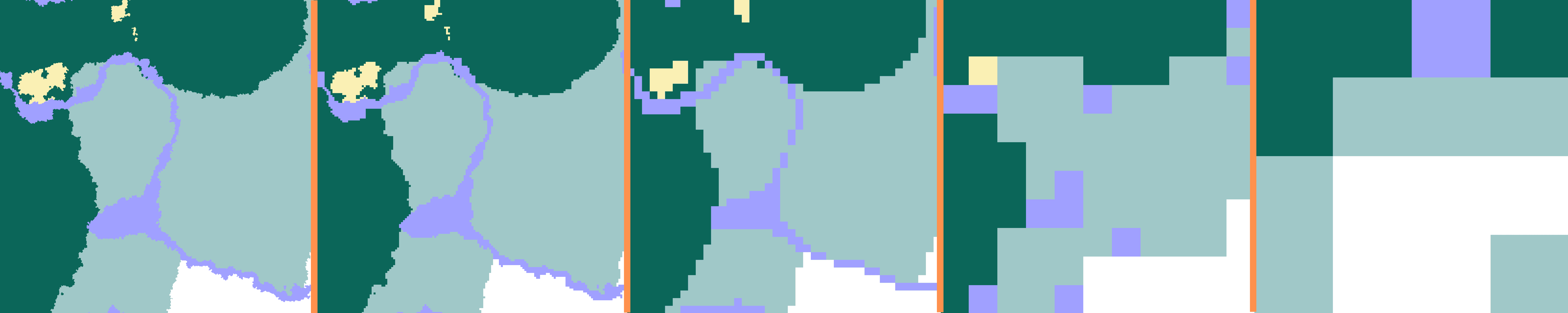
So can we call it a day? Not really. Mapping the world at half-region scale is both highly inaccurate and, frankly, a little… “cheaty”. Doing so would be no better than randomly assigning biomes to each 256×256 block area, since most of the data gets lost.
A better approach is to generate the world at half-region scale initially, then swap in higher-resolution tiles as the player zooms in. Half-regions break down into quad chunks (4×4 chunks), then chunks, then quad blocks (4×4 blocks), and finally individual blocks. This way, we preserve detail where it matters while keeping large-scale rendering efficient.
It is quite apparent that mapping at upto chunk scale (third image) is the best option as it balances accuracy and speed the most.
Performance Scaling
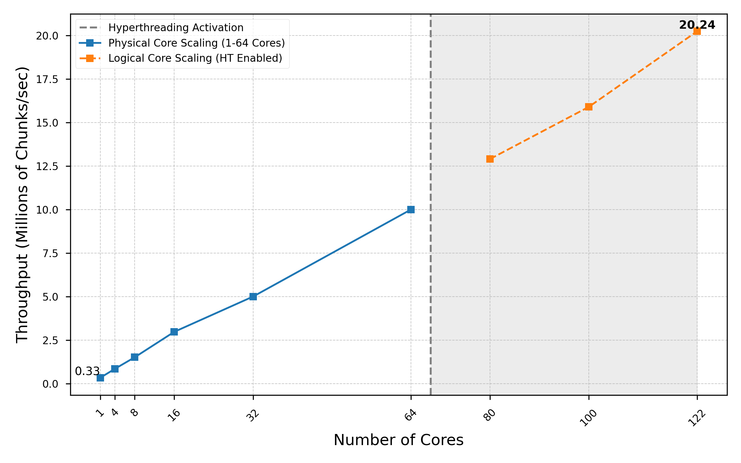
The scaling analysis of this chunk processing workload reveals three distinct performance regimes, reflecting varied efficiency across physical and logical core counts.
The initial performance phase (1 to 8 cores) is characterized by pronounced sub-linear scaling, indicating significant overheads inherent in starting and managing the parallel workload. Moving from 1 core (0.33 million chunks/sec) to 4 cores (1.00 million chunks/sec) results in a 3.03× performance increase, falling short of the ideal 4× factor.
Efficiency dramatically improves after the 8-core mark, with the system achieving near-perfect linear scaling across the majority of the high-end physical core range. The performance increase from 8 to 16 cores (1.51 million to 2.97 million) is almost exactly 2×, and crucially, the efficiency between 32 cores (5.00 million) and 64 cores (10.00 million) is 100%, demonstrating true linear scaling. This indicates that once the initial communication and synchronization barriers are overcome, the chunk processing task is highly parallelizable and optimally utilizes the available physical execution units, confirming that the computational component of the workload is well-distributed.
The final phase, utilizing hyperthreading (logical cores beyond 64), demonstrates exceptional efficiency. Despite the expectation of diminishing returns when sharing physical resources, the system throughput increases from 10.00 million at 64 cores to 20.24 million at 122 cores. This remarkable 102.4% performance boost from the 58 logical cores suggests that the workload is heavily latency-bound (e.g., waiting for data from memory). The logical cores are successfully used to hide these latency periods, ensuring the physical pipelines are kept busy and fully saturated. This superior performance in the hyperthreaded region highlights that the application is not solely compute-bound but benefits greatly from the simultaneous multithreading capabilities of the platform.
Storage and Rendering
Storing output
Once the biome generation process was fully parallelized, an efficient data storage pipeline became critical. Each MPI rank is assigned a section of the world grid and is responsible for generating the biomes for that range. Instead of writing to a single shared file—which could have led to severe I/O contention across nodes, each rank writes to its own binary output file (
00000000 42 49 4F 31 00 00 10 00 00 00 10 00 00 00 00 02 |BIO1............|
00000010 00 00 00 01 00 00 00 00 00 00 00 00 00 00 00 04 |................|
00000020 00 00 00 05 00 00 00 05 00 00 00 03 00 00 00 02 |................|
00000030 00 00 00 00 00 00 00 01 00 00 00 02 00 00 00 02 |................|
00000040 00 00 00 03 00 00 00 04 00 00 00 04 00 00 00 04 |................|
00000050 00 00 00 05 00 00 00 05 00 00 00 05 00 00 00 06 |................|This small binary dump represents the structure of a single .bin biome tile file as generated by the renderer.
The first four bytes (42 49 4F 31) correspond to the ASCII characters BIO1, which act as a magic header identifying this file as a valid biome data file. Following that, a series of 32-bit integers define the scale and the bounding coordinates of the tile — specifically x0, z0, y0, x1, z1, and y1. These determine the section of the Minecraft world that this file covers.
After the header, the remainder of the file is a flat array of 32-bit integers, each representing a biome ID at a specific (x, z) coordinate within that tile. For example, values like
Once all ranks complete, the root process aggregates their contributions using a master index file (biome_index.txt), which serves as a manifest for all generated tiles. This file lists each rank’s coordinate range and its corresponding binary file path. During post-processing, a rendering binary reads this index, loads each tile into memory, and places it at the correct coordinates in a massive global biome grid. The modular tile-based system means that individual tiles can be re-rendered or reprocessed independently, enabling partial updates or region-specific refinements without rerunning the entire generation process.
Rendering the world
Once all biome data files are generated, the renderer stitches them together into a single, continuous map of the Minecraft world. Each .bin file corresponds to a small rectangular region of the world (a tile) and contains raw biome IDs in a tightly packed grid. When the renderer starts, it first reads an index file (
Each tile is then read sequentially. The renderer parses its header to determine its position and size, loads all biome IDs, and looks up the corresponding colors from a predefined biome color map. Every ID — whether it represents an ocean, plains, jungle, or snowy mountain — is mapped to a distinct RGB triplet. These color values are then placed into the correct location within the world image buffer, aligning perfectly based on the tile’s coordinates.
After all tiles have been processed and their colors written, the combined RGB buffer is exported as a PNG using the stb_image_write library. This results in a fully colored top-down biome map, where every pixel represents one block, chunk, or region of the Minecraft world — depending on the selected scale. The final image captures billions of data points in a single view, revealing the entire biome distribution of the world at a glance.
Downsampling
Once the full-resolution biome map has been constructed, the program optionally performs downsampling if the user provides target dimensions via command-line arguments. The method used is a simple nearest-neighbor mapping, where each output pixel corresponds to a specific region of the original image, and its color is directly taken from the closest original pixel. For example, if the original map is 10,000×10,000 and the user requests a 1,000×1,000 output, each downsampled pixel represents a 10×10 block of the source map.
Nearest neighbor interpolation was used to preserve individual pixels in the rendered image. The use of bilinear or cubic interpolation would have resulted in the map being turned into a blurry mess.

In practice, this means the tool can quickly generate overview maps at arbitrary resolutions without sacrificing correctness of biome placement. The downsampled image is saved as biomes_downsampled.png, providing a clear, manageable visualization of the entire world while keeping the computational cost low.
Hardware
This project was executed on a custom-built, small-scale high-performance computing cluster that I helped assemble at Technische Hochschule Deggendorf (THD) under the guidance of Professor Christoph Schober
The cluster currently consists of 5 interconnected nodes, providing a total of 68 physical cores (122 logical CPUs with Hyper-Threading). Each node is a dual-socket system equipped with Intel® Xeon® processors from the E5-2600 v3 family, primarily E5-2620 v3 CPUs, though some nodes include 8-core variants.
- Processor: Dual Intel® Xeon® E5-2620 v3 @ 2.40 GHz (6–8 cores per socket)
- GPU: NVIDIA RTX 3060 (unused for this project, as no GPU acceleration was employed)
- Memory: 32 GB DDR4 RAM per node
- Interconnect: 10 Gbps Ethernet
- Operating System: AlmaLinux 9.6
- MPI Implementation: OpenMPI 5.0.7
While the RTX 3060 GPUs provide potential for future GPU-accelerated projects, the current mapping implementation is entirely CPU-driven, relying solely on distributed parallelism across the MPI ranks.
Despite the modest hardware configuration and relatively slow interconnect, the system demonstrated exceptional parallel scalability, efficiently saturating all logical cores during full-world biome generation. This validates the MPI-based design and efficient caching strategy — proving that massive-scale biome rendering is achievable even on mid-range academic clusters.
The Map
At the very start of this project, using the original Cubiomes implementation, the system could process only ~0.18 million chunks per second. At that rate, generating even 1% of the full Minecraft world which would roughly be 140 billion chunks would have taken more than nine days of continuous computation. With all the optimizations, parallelization, and caching improvements described throughout the blog series, throughput was eventually pushed to over 20 million chunks per second, reducing that same 1% mapping task from about nine days to under two hours on the cluster.
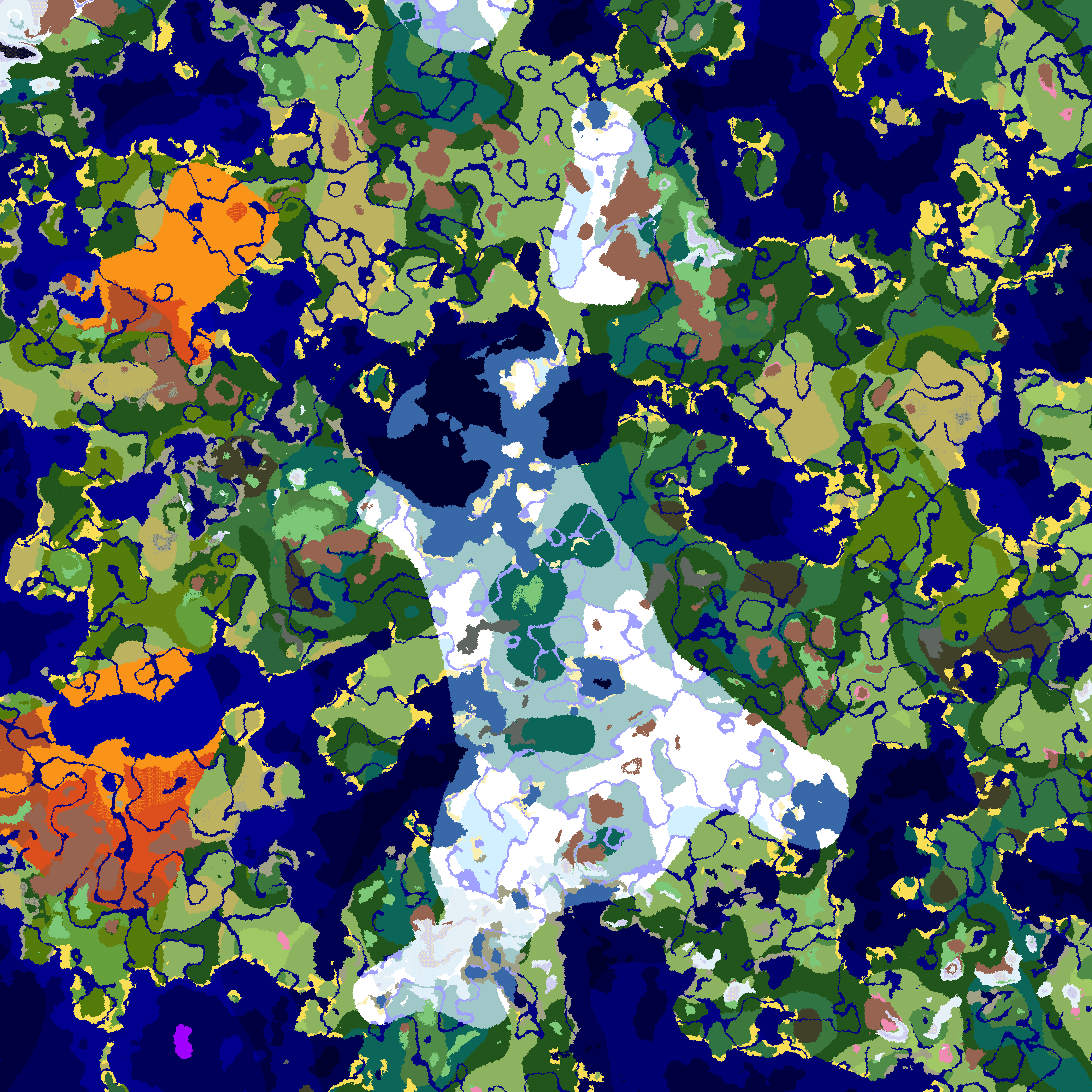
Here is a downsampled preview of 1% area of a complete Minecraft world map. While the full-resolution version would be a staggering 160K×160K pixels (over 25 billion pixels) and weigh in at several terabytes, this 16K×16K preview already demonstrates the incredible scale and detail of the complete biome distribution. The full map would be impractical to host, download, or view on most systems—but the beauty of open source is that anyone can generate their own complete world map using the code and techniques described in this series. Simply run the renderer with your desired resolution and watch as the entire Minecraft world unfolds before you.

Conclusion
And with that, the project finally comes to an end.
It started as a small side experiment, just an attempt to see how far Minecraft’s procedural generation could be pushed, and it turned into something far more interesting than I ever expected. It was never meant to be anything special, but along the way it became a deep dive into distributed computation, optimization, and the art of scaling performance. The repository in its final state can be found here.
This project made it possible to generate biome maps at unprecedented speeds, which is something that once seemed completely out of reach. Beyond the technical success, it also opened up a fascinating line of inquiry into linear scaling behavior under hyperthreading, which I’m now developing into a formal research paper.
This marks the conclusion of the Ultrafast Minecraft Biome Generation series. It’s been an incredibly rewarding learning experience and it taught me more about parallelism, performance tuning, and system design than I anticipated. Now, it’s time to move on to new projects, new challenges, and new worlds to explore.